Ecological Archives A025-005-A1

D. Stralberg, S. M. Matsuoka, A. Hamann, E. M. Bayne, P. Sólymos, F. K. A. Schmiegelow, X. Wang, S. G. Cumming, and S. J. Song. 2015. Projecting boreal bird responses to climate change: the signal exceeds the noise. Ecological Applications 25:52–69. http://dx.doi.org/10.1890/13-2289.1

Appendix A. Global climate model summary and downscaling methods.

Downscaling Methods

Global climate model (GCM) projections were obtained from the Intergovernmental Panel on Climate Change (IPCC) 4th Assessment Report (AR4) (IPCC 2007) as part of the World Climate Research Programme's Coupled Model Intercomparison Project phase 3 (WCRP CMIP) multi-model dataset [http://www-pcmdi.llnl.gov/ipcc/info_for_analysts.php] (Meehl et al. 2007). Historical projections were taken from the 20th century simulation, which were generally initiated between 1850 and 1880 and run through 1999 or 2000. Future projections were taken from three emission scenarios (IPCC 2000)—SRESA2 (high), SRESA1B (intermediate), and SRESB2 (low)—run from 2000 or 2001 through at least 2099 or 2100. Projections of monthly temperature and total precipitation were averaged across multiple GCM runs (if available) for each thirty-year period. A total of 24 GCM simulations were used, 17 of which were run for all three future scenarios, with grid cell resolutions ranging from 1.125° to 5° (Table A2). Temperature values were converted to degrees Celsius and precipitation values were converted to mm/day.

For each future time period, we calculated climate anomalies as the absolute change in temperature and the percentage change in precipitation between the projected values for each future period and the projected climate normals for the baseline period. Projected precipitation anomalies were capped at 500% of the projected normal to prevent unrealistic values stemming from chance differences at the low end of the precipitation spectrum. We clipped the projected climate anomalies to North America, downscaled them to a 0.5° resolution using a thin-plate spline interpolation, and then added the downscaled anomalies to the 4-km interpolated climate normals (described above). We did not have future projections for minimum and maximum temperature for 13 of the 19 GCMs. We therefore used the average temperature anomalies in place of minimum and maximum temperature anomalies to calculate future projected minimum and maximum temperature averaged across GCMs. Mean monthly projections of monthly temperature and precipitation were used to calculate derived bioclimatic variables (Table A1) for each 4-km grid cell in each future time period. Projections for each variable and each time period (including current baseline) were converted to separate raster layers for GIS analysis and mapping purposes.

Technical details

GCM projections in NetCDF format were imported into R and manipulated into a tabular format using the 'ncdf' (Pierce 2013) package. Due to inconsistent time periods across GCMs, the starting year for each simulation was included in the NetCDF file name for parsing purposes. For each GCM run and for each variable (tmin, tmax, tavg, prec), a separate .csv file for each simulation year was created, with one record per grid cell (as given by x-y coordinates) and one column per month. Annual monthly means were then averaged across 30-year time periods, creating a single .csv file for each 30-year time period. In this step, longitude coordinates were converted from a scale of 0–360 to a standard geographic coordinate system (central meridian at Greenwich) ranging from -180 to 180.

Anomalies were converted to raster format using the 'raster' package, and clipped to the North American land boundary. Remaining points were interpolated with a thin-plate spline algorithm using the 'fields' (Fields Development Team 2006) and 'raster' (Hijmans and van Etten 2012) packages. Interpolated monthly anomalies for each future period were added to the baseline (1961-1990) monthly means to create .csv files containing monthly mean projections for centerpoints of a 4-km grid for North America. These monthly projections were then used to calculate a separate csv file containing derived bioclimatic variables for each future period.

Finally, decimal-degree-based projections for monthly and derived bioclimatic variables were joined with a base file containing Lambert Conformal Conic coordinates using a unique identifier field. Points outside of the 4-km grid (small protected areas) were filtered out, and separate .asc raster layers (4-km grid cell resolution) were generated for each variable using the 'raster' package.

We performed all climate data manipulations using the program R, version 2.12.1 (R Development Core Team 2010).

Literature Cited

Chen, W., Z. Jiang, and L. Li. 2011. Probabilistic projections of climate change over China under the SRES A1B scenario using 28 AOGCMs. Journal of Climate 24:4741–4756.

Fasullo, J. T., and K. E. Trenberth. 2012. A less cloudy future: the role of subtropical subsidence in climate sensitivity. Science 338:792–794.

Fields Development Team. 2006. fields: Tools for Spatial Data. National Center for Atmospheric Research, Boulder, CO. Available on-line at http://www.cgd.ucar.edu/Software/Fields.

Gleckler, P. J., K. E. Taylor, and C. Doutriaux. 2008. Performance metrics for climate models. Journal of Geophysical Research 113:D06104.

Hijmans, R. J., and J. van Etten. 2012. Package 'raster'. Available on-line at http://cran.r-project.org/web/packages/raster/index.html

Hogg, E. H. 1997. Temporal scaling of moisture and the forest-grassland boundary in western Canada. Agricultural and Forest Meteorology 84:115–122.

IPCC. 2000. Special Report on Emissions Scenarios. Summary for Policymakers. A Special Report of IPCC Working Group III.

IPCC. 2007. Climate Change 2007: The Physical Science Basis. Contribution of Working Group I to the Fourth Assessment Report of the Intergovernmental Panel on Climate Change. Cambridge University Press, Cambridge, UK.

Meehl, G. A., C. Covey, T. Delworth, M. Latif, B. McAvaney, J. F. B. Mitchell, R. J. Stouffer, and K. E. Taylor. 2007. The WCRP CMIP3 multi-model dataset: a new era in climate change research. Bulletin of the American Meteorological Society 88:1383–1394.

Pierce, D. 2013. Package 'ncdf'. Available on-line at http://cran.r-project.org/web/packages/ncdf/index.html.

R Development Core Team. 2010. R: A language and environment for statistical computing. R Foundation for Statistical Computing, Vienna, Austria.

Scherrer, S. C. 2011. Present-day interannual variability of surface climate in CMIP3 models and its relation to future warming. International Journal of Climatology 31:1518–1529.

Walsh, J. E., W. L. Chapman, V. Romanovsky, J. H. Christensen, and M. Stendel. 2008. Global climate model performance over Alaska and Greenland. Journal of Climate 21:6156–6174.

Wang, M., J. E. Overland, V. Kattsov, J. E. Walsh, X. Zhang, and T. Pavlova. 2007. Intrinsic versus forced variation in coupled climate model simulations over the Arctic during the twentieth century. Journal of Climate 20:1093–1107.

.Table A1. Summary of derived bioclimatic variables calculated for 24 GCMs, three emission scenarios, and four time periods.

¹ Calculated using Hogg's (1997) modified Penman-Monteith method. Values were calculated separately for each month and then summed across months of interest.

Table A2. General circulation models (GCM) and country of origin, their spatial resolution, and their associated number of runs for each century and climate variable. The projected climate variables include monthly precipitation (precip) and monthly average (tavg), minimum (tmin), and maximum (tmax) temperature. The four climate models in bold are compared herein. Models below the dotted line were not candidates for selection.

¹ 20°–90°N: precipitation, temperature, sea level pressure

² Arctic: inter-annual variability

³ 20°–90°N

⁴ China: spatial accuracy, inter-annual variability

⁵ Inter-annual variability

⁶ Subtropics: cloud dynamics, moisture

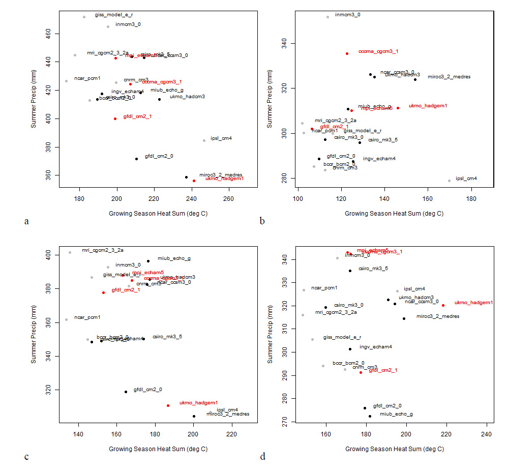
Fig. A1. Global climate model (GCM) differences: growing season heat sum (growing degree days above 5 °C) vs. mean summer precipitation (mm) for 19 GCMs based on the A2 emissions scenario for 2071–2100. Values are summarized by level 1 ecoregions as defined by the Commission for Environmental Cooperation: (a) Northern Forests, (b) Taiga, (c) Hudson Plains, (d) Northwest Forested Mountains. GCMs chosen for analysis are shown in red. Models not considered are shown in gray.

[Back to A025-005]