Appendix B. Habitat clusters, obtained from different altitude ranges using the SEL variable subset, projected on the first and second discriminant axes.
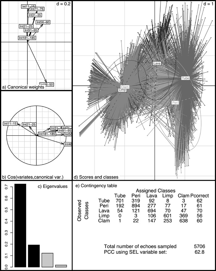
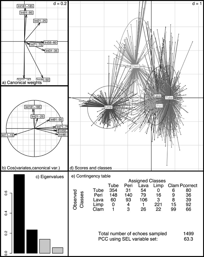
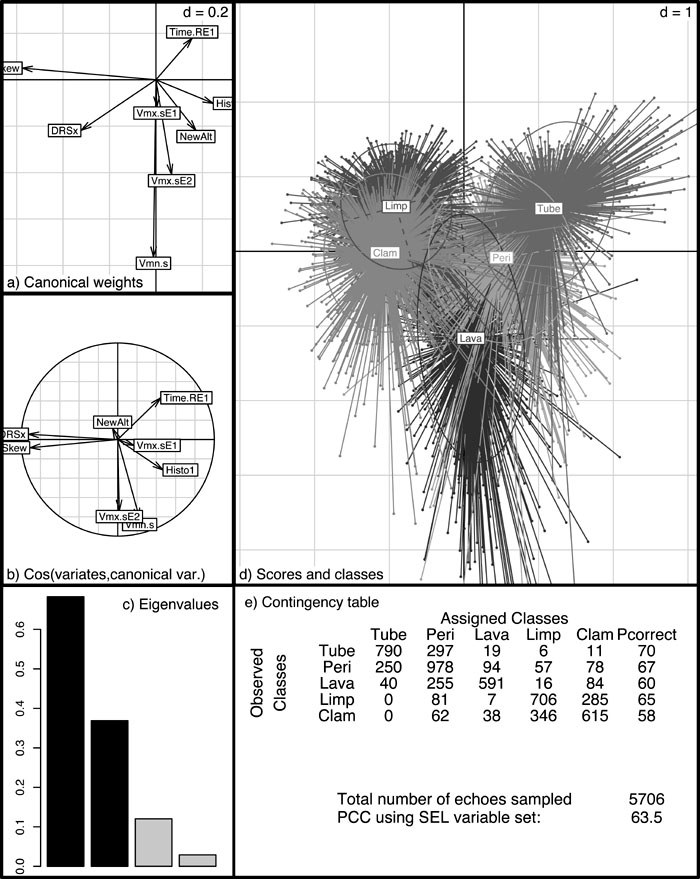
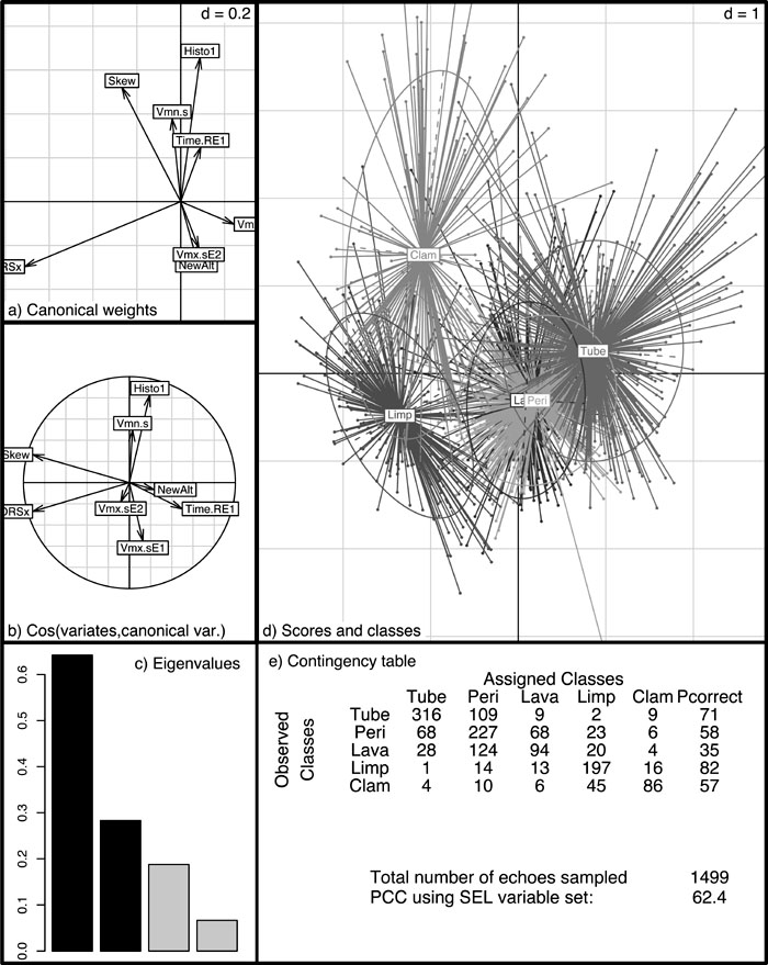
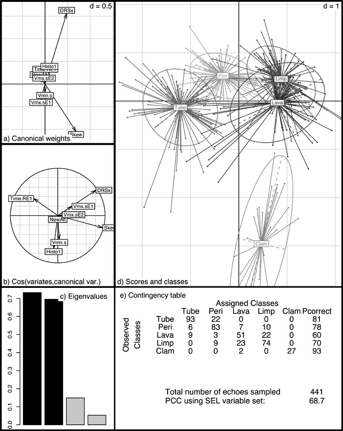
The SEL subset of variables was used to construct the six figures presented in this Appendix. The first three figures (Fig. B1, Fig. B2, Fig. B3) are based on the VI data tables (power intensity values found in the echoes) whereas the following three (Fig. B4, Fig. B5, Fig. B6) on the VE data tables (variables describing echo shapes). VT graphs are not shown since the nature of their variable sets (VI and VE combined) makes it harder to unravel the links and relationships between the variables and the centroids of the habitat clusters created by discriminant analysis (R-Pkg::ade4:Discrimin). In each figure, 4 panels (a to d) and one table (e) are shown. In panels (a) to (d), discriminant axis 1 is the abscissa and axis 2 is the ordinate. Panel (a) shows the canonical weights of the variables; panel (b) shows the variables at angles representing their correlations relative to the first two discriminant axes; in panel (c), the eigenvalues of the first four discriminant axes are shown. Panel (d) shows the sonar return clusters based on their video-assigned habitat types; for each habitat cluster, the nametag is located at the cluster centroid. In panel (e), the classification table compares the habitats assigned by discriminant analysis (columns) to the video-assigned habitats (rows). PCC is the percentage of correct classification. In panels (d), the Limp and Clam habitats are always visually well-separated from the other habitat clusters. The habitat assignations in the contingency tables of Figs. B1, B2, B4, and B5 also differentiate these two major groups. It is only in Figs. B3 and B6, which describe echoes acquired between 7 and 10 m of altitude, that most echoes are correctly assigned.
All selected VI variables described in panels (a) and (b) of Figs. B1 to B3 have, at one altitude range or another, shown a high canonical weight or correlation with one of the axes. This behavior suggests that VI is a good variable set for habitat classification. When the VE variables are used (Figs. B4–B6), the "Skew" and "DRSx" variables, which always have strong correlations and canonical weights with the axes, played influential roles in our discrimination results. They allowed us to identify the sonar signatures of the five dominant habitats found in a hydrothermal vent field, 2200 m below the sea surface.
|
|
| FIG. B1. Table of variables VI, subtable 1–4 m. |
|
| FIG. B2. Table of variables VI, subtable 4–7 m. |

|
| FIG. B3. Table of variables VI, subtable 7–10 m. |
|
| FIG. B4. Table of variables VE, subtable 1–4 m. |
|
| FIG. B5. Table of variables VE, subtable 4–7 m. |
|
| FIG. B6. Table of variables VE, subtable 7–10 m. |