Appendix B. Description of the individual-based model used to simulate the frequency distributions of instantaneous and lifetime fecundities in a population of the Mediterranean shrub Lavandula latifolia.
To facilitate repeatability, the description below follows the ODD (“Overview, Design concepts, and Details”) protocol for individual- and agent-based models proposed by Grimm and Railsback (2005) and Grimm et al. (2006). The model is implemented in NetLogo 4.0.3 (Wilensky 1999; downloadable from http://ccl.northwestern.edu/netlogo/download.shtml), and the code is available in the Supplement.
Purpose.—The model does not pretend to be a realistic representation of either the physiology of plants or the intra- and interespecific interactions, nor it is aimed to reproduce the real magnitude of the number of actively growing branch tips (termed “modules” for simplicity; Nmodules) or inflorescences (Ninflorescences) found in the studied population. Rather, the purpose of the model was to produce a sketch of the system enabling us to explore the power of multiplicative growth (dichasial, dichotomous branching) of L. latifolia plants, acting in concert with stochastic environmental variation, on shaping the instantaneous and lifetime distributions of individual fecundity.
State variables and scales.—The entities of the model are 1,000 individuals of a virtual L. latifolia population. Each plant is characterized by its Nmodules, and the Ninflorescences produced. One time step of the model corresponds to one yr; simulations are run until all the individuals die (after ca. 25 yr). Environmental variables are described as a stochastic process both in space and time.
Process overview and scheduling.— Every time step, the Nmodules of each plant is updated according to its Nmodules on the preceding yr, the environmental conditions shaping its growth and a senescence factor that linearly lowers the production of new modules. Ninflorescences result from current Nmodules and the environmental conditions affecting its production.
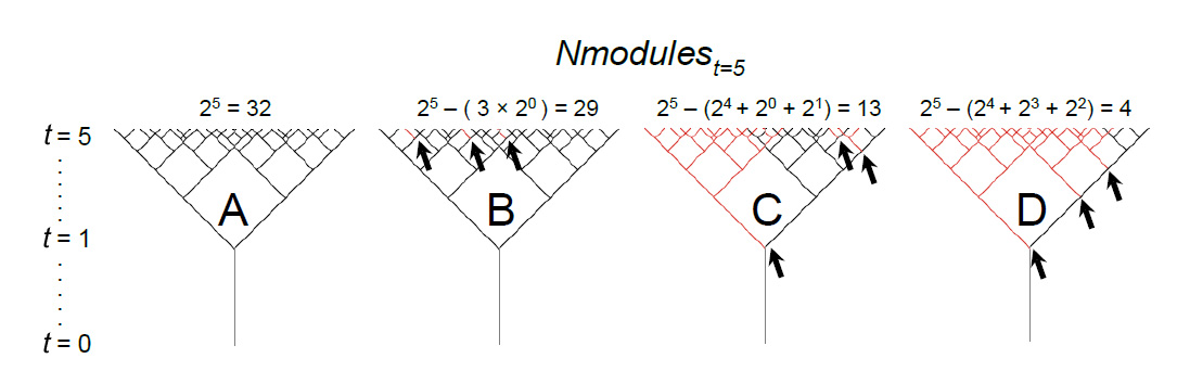
Design concepts.—Instantaneous and lifetime distributions of individual fecundity emerge from the modular growth and stochastic environmental factors lowering the maximum growth potential of each plant. The dichasial growth of L. latifolia implies a potential multiplicative increase on the maximum Nmodules such as 2t, being t the age in yr of the plant. That is, plants start with 1 module in yr 0 and their maximum potential Nmodules increase multiplicatively such as 2, 4, 8, 16, 32 , ... (Fig B1). This multiplicative growth also implies that environmental factors can potentially create a long-lasting effect on the fecundity of plants depending on the timing of harmful environmental effects (see Fig B1).
|
|
| FIG. B1. Harmful effects of environmental stochasticity amplify multiplicatively through the years. Black segments between nodes illustrate modules (e.g., in plant A the Nmodules increase by 2t, from 1 module in yr 0 to 32 modules in yr 5). Black arrows show the effect of one environmental factor precluding the creation of one module. Red segments illustrate modules that have never existed because (1) directly suffered the harmful effect of environmental stochasticity before producing an inflorescence or (2) indirectly by lacking a preceding module to produce them. Thus, a single harmful episode precludes the potential growth of complete plant portions, multiplicatively (i.e., 2t Nmodules) increasing its harmful effect yr after yr. For instance, plants B–D, each suffered three damaging environmental events. However, the consequences were dramatically different for the final Nmodules at t = 5 for each plant (and the potential corresponding Ninflorescences growing from them) according to the timing of harmful events; C and particularly D are more affected because of the earlier occurrence of such detrimental episodes. |
All individuals are initially identical (clones) and grow in a homogeneous environment. Thus, differences in instantaneous and lifetime fecundities originate only because of environmental stochasticity occurring at different rates and at different times through the life of each plant. To observe the model output, we looked at the instantaneous and lifetime distributions of individual fecundity in the population.
Initialization.— Simulations are initialized (at yr t = 0) with 1,000 plants with one module each one.
Input.— The model has not an external input; environmental variables are created stochasticly.
Submodels.—The model has two submodels describing the growth in Nmodules of each plant from year to year and the production of Ninflorescences from the Nmodules in the current year.
Because of the fork branching of L. latifolia, the maximum Nmodules is the double of the number of modules the yr before [i.e., max(Nmodulest) = 2 x Nmodulest-1] (Fig B1). However, natural conditions for plant growth are often lower than this optimal due to an array of biotic and abiotic factors with different temporal and spatial scales, e.g. soil nutrients, intra and intererspecific interactions, rain, insolation. For instance, the fall of a stone can have spatially local and temporally permanent effects on a given plant, but rain or wind can have (spatially) homogeneous and (temporally) punctual effects on all the plants of a given population. Here, we modelled the most stochastic possible scenario - environmental factors being independent in space and time. That is, environmental factors affecting modular growth and production of inflorescences are independent both within plants within yr, between different plants in a given moment and between plants in different yr. We summarized this environmental-stochasticity by extracting a pseudorandom number from a uniform distribution between 0.6 and 1. Each yr, and for each plant, a different environmental-stochasticity value shaped the production of modules and the production of inflorescences.
Senescence was introduced as a linear decrease on the probability of survival of each module from one yr to the next. Assuming a maximum age of 32 yr for the individuals of the study population (C. M. Herrera, unpublished data), we introduced senescence into the model as ( 1 - ( t / 32 ) ), that is, each yr a fraction yr/32 of modules die due to senescence processes that occur independently of the other factors considered. The assumption of a linear senescence function is a conservative approach, as it only assumes that the effects of senescence increase linearly with age, and avoids imposing on the results of the simulation any particular timing for the start of senescence. Overall, each yr the Nmodules (rounded to the nearest integer) is updated for each plant as follows:
| Nmodulest = 2 × Nmodulest-1 × ( 1 - ( t / 32 ) ) × environmental-stochasticity | (B.1) |
| Ninflorescencest = Nmodulest × environmental-stochasticity | (B.2) |
LITERATURE CITED
Grimm, V., and S. F. Railsback. 2005. Individual-based modeling and ecology. Princeton University Press, Princeton, New Jersey, USA.
Grimm, V., U. Berger, F. Bastiansen, S. Eliassen, et al. 2006. A standard protocol for describing individual-based and agent-based models. Ecological Modelling 198:115–126.
Wilensky, U. 1999. Netlogo. Center for Connected Learning and Computer-Based Modeling, Northwestern University, Evanston, Illinois, USA. See http://ccl.northwestern.edu/netlogo.