Jonathan A. Hare, Michael A. Alexander, Michael J. Fogarty, Erik H. Williams, and James D. Scott. 2010. Forecasting the dynamics of a coastal fishery species using a coupled climate–population model. Ecological Applications 20:452–464.

Appendix A. Background on general circulation models, choice of a stock–recruitment function, and distribution model based on logistic regression.

1. Background on general circulation models

Annual minimum monthly winter air temperature was derived from 14 General Circulation Models (GCMs, Table A1). Also known as global climate models, GCMs depict the climate using a three dimensional grid over the globe, typically with horizontal resolutions between 250 and 600 km, 10 to 20 vertical layers in the atmosphere, and as many as 30 layers in the oceans. The resolution of these models is coarse and subgrid scale processes (e.g., turbulence in the boundary layer, thunderstorms and ocean eddies) are parameterized based on large-scale conditions, i.e., variables that are simulated on the model’s coarse grid. Even at coarse resolution, the models are run on super computers as the temperature, moisture, salinity, winds, ocean currents, etc., are predicted at hundreds of thousands of grid boxes.

GCMs can be verified by comparing their output to the recent past, e.g., how simulated and observed temperatures changed over the 20th century. An exact match between observations and model simulations in a given period is not expected because of random fluctuations in the climate system. To overcome the influence of these random fluctuations, the output of an ensemble of model runs (as opposed to a single model run) is generally compared to observations.

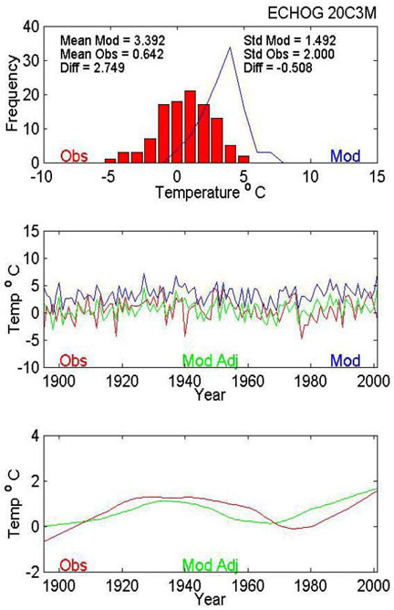
All the GCMs used here have simulations for the 20th century. Annual minimum monthly winter temperatures (minimum[Dec, Jan, Feb, and Mar]) for the grid cell over southern Chesapeake Bay was extracted from the 20th century runs and compared with observed minimum winter temperatures for Virginia (http://www.sercc.com/climateinfo_files/monthly/Virginia_temp.html). As an example, the GFDL CM2.1 mean was about 0.5°C lower and the standard deviation was slightly greater than observed (Table A2). The mean differences of other models ranged from +10°C to –4°C. These mean differences between the climate models and observations were used to bias correct the minimum winter air temperatures estimated by each GCM. The smoothed observations indicate a long-term cycle in minimum winter air-temperature with high temperatures in the 1940’s and low temperatures in the 1970’s; these warm and cool periods have been linked to the Atlantic Multidecadal Oscillation (Kerr 2000, 2005). Some of the modeled temperatures do not match this long-term trend in observed temperature, and many of the modeled temperatures seem to exhibit a cycle of similar frequency and magnitude as observed but with different timing.

TABLE A1. List of General Circulation Models (GCMs) used in this study. The institution and model name are provided, as are the links to the model metadata. For each GCM, three scenarios were used: commit, B1, and A1B. In addition, a 20th century simulation was compared to 20th century observations to develop a mean bias correction for each model. All model outputs were downloaded from the World Data Center for Climate, IPCC Data Distribution Centre (http://www.mad.zmaw.de/IPCC_DDC/html/SRES_AR4/index.html)

TABLE A2. Mean correction bias for each GCM. The average simulated minimum winter air temperature was compared to the average observed minimum winter air temperature over the 20th century. The difference in averages was added to the GCM simulated minimum winter air temperatures. A comparison of standard deviations is also provided.

FIG. A1. Distributions of observed and modeled reanalysis minimum winter air temperatures and comparison of observed and predicted means and standard deviations of temperature (top row). Time series of observations and GCM predicted minimum winter temperatures. Also shown is the corrected model estimate based on adding the mean model vs. observation difference to the model. Smoothed observations and predictions, with the predictions corrected by the mean difference between model and observations (bottom row). Results are shown for the ECHOG GCM; similar analyses were done for all GCMs. Observations are minimum monthly winter temperature in Virginia and model results are from the grid cell encompassing Chesapeake Bay.

Prior studies have shown that GCMs generally reproduce the continental-scale trends (Randall et al. 2007) and some regional trends (Knutson et al. 2006, Seager et al. 2007). For example, the GFDL CM2.1 reproduces the observed warming over the 20th century in the subtropical North Atlantic and continental U.S. when anthropogenic forcing is included, but over-estimates warming for the southeast U.S. (Knutson et al. 2007). All climate models have biases and several factors may lead to model-data differences including model error, inadequate representation of regional processes (e.g., aerosol loading, deforestation/reforestation, irrigation), and natural variability (i.e,. the atmospheric circulation over the southeast United States is influenced by El Nino and the Atlantic Multidecadal Oscillation). While there are differences between the GFDL CM2.1 and the observed annual temperature trends in the southeast U.S., there is general agreement between the simulated and observed minimum winter temperature in the GCMs considered here (Fig. A1 and Table A2).

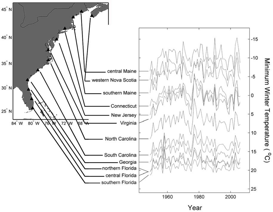
Although, the analyses above suggest that the climate models reasonably capture the minimum monthly winter air temperatures in coastal Virginia, a potential concern is that the coupled climate–population model results are specific for this model grid cell. However, there is strong concordance in the time series of minimum winter air temperature over the eastern seaboard of the United States in historical observations and climate model hindcasts (Fig. A2 and Table A3). This concordance is expected since prior studies have documented strong concordance in interannual winter air temperature over the eastern U.S. (Joyce 2002), estuarine water temperatures in the mid-Atlantic (Hare and Able 2007), coastal water temperatures (Nixon et al. 2004), and sea surface temperature in the western North Atlantic (Friedland and Hare 2007). Additionally, minimum winter air temperature is closely related to minimum winter water temperature in estuaries along the mid-Atlantic coast (Hettler and Chester 1982, Hare and Able 2007) owing to the efficient heat exchange between atmosphere and water in these shallow systems (Roelofs and Bumpus 1953). Thus, minimum winter air temperatures from Virginia can serve as a proxy for coast-wide variability in minimum winter water temperatures.

FIG. A2. Time series of minimum winter air temperatures from the NCEP Reanalysis for grid cells nearest the locations indicated on the map. These data were significantly concordant: the pattern of interannual variability was coherent across the time series.

TABLE A3. Kendall’s concordance (W) for time series of minimum winter air temperatures from locations indicated in Fig. A3. Calculations were made for each of the models considered based on the 20th century runs. Kendall’s concordance is a non-parametric test that measures the degree of agreement between multiple series of data: 0 indicates no agreement; 1 indicates perfect agreement. The NCEP/NCAR Reanalysis Product was also included in these analyses. This product is a gridded data set based on retrospective observations (1948–2006) of a variety of atmospheric variables including surface temperature (Kalnay et al. 1996).

2. Choice of a stock-recruitment function

A number of functions have been used historically to model the relationship between fish population size and subsequent recruitment (Hilborn and Walters 2004). There also are a number of extensions of these functions that include the effect of the environment on recruitment (Hilborn and Walters 2004). We evaluated two common stock recruitment functions (Beverton-Holt and Ricker) and several extensions of these functions that include environmental effects (Table A4). The Akaike Information Criterion (AIC) was used to choose the best formulation for the coupled climate–population model. Spawning stock biomass and recruitment data were obtained from a recent stock assessment of Atlantic croaker (ASMFC 2005) and minimum winter air temperature in Virginia (http://www.sercc.com/climateinfo_files/monthly/Virginia_temp.html) was used as a proxy for water temperature during the estuarine juvenile stage (Hare and Able 2007).

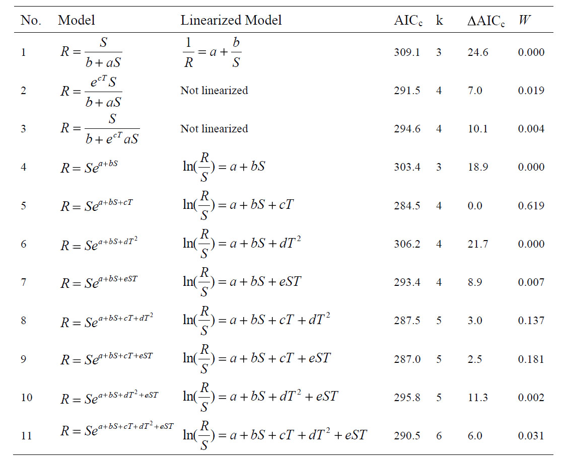
The stock–recruitment functions were initially fit with nonlinear algorithms, but these algorithms rarely converged. As a result, linear forms of the stock–recruitment functions (model 1 and 4, see Table A4) were fit using least-squares regression. The environmental extensions of the Ricker stock–recruitment model are easily linearized (models 5–11, see Table A4) and these models were also fit using least-squares. The environmental forms for the Beverton-Holt model (models 2 and 3) are not easily linearized. To fit these models, the standard Beverton-Holt terms (a and b) were estimated using the linearized version of the model (model 1), and then a nonlinear fitting algorithm was used to estimate the environmental parameter (c) with the standard parameters (a and b) fixed at the appropriate values. Because the linearized forms of the models used different dependent variables (1/R for Beverton and Holt and ln[R/S] for Ricker), AIC was estimated based on the models predictions of R using the non-linearized forms of the equations, with the terms derived from the linearized models. In this way, AIC was calculated based on the residual sums of squares of estimated R and observed R. The strength of evidence of the alternative models was calculated following Burnham and Anderson (1998). The Ricker stock–recruitment model with a temperature term was the best-supported model evaluated (Table A4), with the highest strength of evidence (w = 0.619). The models with environmental terms were far superior to the standard stock–recruitment models. The relative likelihood of the environmental Beverton and Holt model (model 2) compared to the standard Beverton and Holt model was ~6000 to 1 (w_{model 2} / w_{model 1}). For the environmental Ricker (model 5) compared to the standard Ricker (model 4), the relative likelihood was ~10000 to 1. Based on these results, model 5 was chosen for use in the population model. Temperature-dependent Ricker models with higher order terms (model 8 and 9) had moderate strengths of evidence (w = 0.137 and w = 0.181). Model 8 includes a T² term, which could amplify the effect of warming on recruitment at higher minimum winter temperatures. However, over the range of temperatures forecasted in the climate models, the higher order models (model 8 and 9) predict very similar recruitment compared to the linear model (model 5), so nonlinear effects are minimal, and thus these were not included in the final model.

TABLE A4. Akaike Information Criteria values for various models fit to stock (S) and recruitment (R) data for the mid-Atlantic stock of Atlantic croaker. Values provided for corrected Akaike Information Criteria (AIC_c), number of parameters in the model including the error term (k), the delta-AIC_c, which is scaled to the minimum observed AIC_c, and the model weights (w), which range from 0 to1.

3. Distribution model based on logistic regression

A multivariate regression approach was used to model distribution as a function of population size and winter temperature. The hypothesis was that as population size increased and winter temperatures increased the mean and northern extent of the population (mean + 2 standard deviations) would shift northward. A shift in mean location is not necessarily predicted with increasing population size; the mean could remain stationary and the northern and southern extents of the population could expand. However, in the case of Atlantic croaker, sampling to determine distribution did not occur throughout the range of the population; sampling stopped at a fixed geographic location, so an expansion in the southern range would not be observed. Thus as the northern range extends and the southern boundary of sampling remains stationary, a northward shift in the mean location is predicted.

As an alternative approach to multiple regression for modeling distribution, a logistic regression was developed that used the presence / absence at individual trawl stations. First, trawl stations were screened to remove stations that sampled deeper than 45 m; this value was based on the 5% level of a logistic regression of catch on depth. In the logistic regression model, catch at station s in year Y was modeled as the distance of station s in year Y, spawning stock biomass (S) in year Y, and minimum winter temperature in year Y:

The model was fit using the glm [family=binomial(link="logit")] function in R (http://www.r-project.org/) and an Akaike multi–model inference was used to determine the model parameters. The model was then used to forecast Atlantic croaker distribution estimating the distance to the 50% and 10% catch probability. The results were qualitatively similar to those from the average distance approach, with distances decreasing with increasing F and increasing with increasing CO₂ emissions; we choose to present the results of the multiple regression model.

LITERATURE CITED

ASMFC (Atlantic States Marine Fisheries Commission). 2005. Atlantic croaker stock assessment and peer-review reports. Atlantic States Marine Fisheries Commission, Washington, D.C., USA.

Burnham, K. P., and D. R. Anderson. 1998. Model selection and multimodel inference: a practical information-theoretic approach. Springer, New York, New York, USA.

Friedland, K. F., and J. A. Hare. 2007. Long-term trends and regime shifts in sea surface temperature on the continental shelf of the northeast United States. Continental Shelf Research 27:2313–2328.

Hare, J. A., and K. W. Able. 2007. Mechanistic links between climate and fisheries along the east coast of the United States: explaining population outbursts of Atlantic croaker (Micropogonias undulatus). Fisheries Oceanography 16:31–45.

Hettler, W. F., and A. J. Chester. 1982. The relationship of winter temperature and spring landings of pink shrimp, Penaeus duorarum, in North Carolina. Fishery Bulletin 80:761–768.

Hilborn, R., and C. Walters. 2004. Quantitative fisheries stock assessment-choice, dynamics and uncertainty Kluwer Academic Publishers, Norwell, Massachusetts, USA.

Joyce, T. M. 2002. One hundred plus years of wintertime climate variability in the eastern United States. Journal of Climate 15:1076–1086.

Kalnay, E., M. Kanamitsu, R. Kistler, W. Collins, D. Deaven, L. Gandin, M. Iredell, S. Saha, G. White, J. Woollen, Y. Zhu, A. Leetmaa, R. Reynolds, M. Chelliah, W. Ebisuzaki, W. Higgins, J. Janowiak, K. C. Mo, C. Ropelewski, J. Wang, R. Jenne, and D. Joseph. 1996. The NCEP/NCAR 40-Year Reanalysis Project. Bulletin of the American Meteorological Society 77:437–471.

Kerr, R. A. 2000. A North Atlantic climate pacemaker for the centuries. Science 288:1984–1986.

Kerr, R. A. 2005. Atlantic climate pacemaker for millennia past, decades hence? Science 309:43–44.

Knutson, T. R., T. L. Delworth, K. W. Dixon, I. M. Held, J. Lu, V. Ramaswamy, M. D. Schwarzkopf, G. Stenchikov, and R. J. Stouffer. 2006. Assessment of Twentieth-Century regional surface temperature trends using the GFDL CM2 coupled models. Journal of Climate 10:1624–1651.

Nixon, S. W., S. Granger, B. A. Buckley, M. Lamont, and B. Rowell. 2004. A one hundred and seventeen year coastal water temperature record from Woods Hole, Massachusetts. Estuaries 27:397–404.

Randall, D. A., R. A. Wood, S. Bony, R. Colman, T. Fichefet, J. Fyfe, V. Kattsov, A. Pitman, J. Shukla, J. Srinivasan, R. J. Stouffer, A. Sumi, and K. E. Taylor. 2007. Cilmate Models and Their Evaluation. in S. Solomon, D. Qin, M. Manning, Z. Chen, M. Marquis, K. B. Averyt, M. Tignor, and H. L. Miller, editors. Climate Change 2007: The Physical Science Basis. Contribution of Working Group I to the Fourth Assessment Report of the Intergovernmental Panel on Climate Change. Cambridge University Press, Cambridge, United Kingdom and New York, NY, USA.

Roelofs, E. W., and D. F. Bumpus. 1953. The hydrography of Pamlico Sound. Bulletin of Marine Science of the Gulf and Caribbean 3:181–205.

Seager, R., M. F. Ting, I. Held, Y. Kushnir, J. Lu, G. Vecchi, H. P. Huang, N. Harnik, A. Leetmaa, N. C. Lau, C. H. Li, J. Velez(Miller), N. Naik, and -. Science. 2007. Model projections of an imminent transition to a more arid climate in southwestern North America. Science 316:1181–1184.